Excel in "Microsoft Excel": Pivot Tables

A Pivot Table is way to present information in a report format. The idea is that you can click drop down lists and change the data that is being displayed. For example, choose just one student from a drop down list and view only his or her scores.

Pivot tables are a lot easier to grasp when you see them in action.

Here's the one we're going to create in this section:

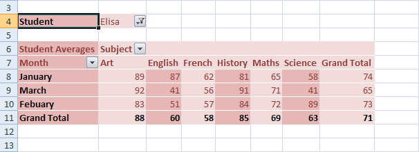
Look at Row 4. This shows that the student is Elisa. If we click Elisa's drop down arrow, we'll see this:

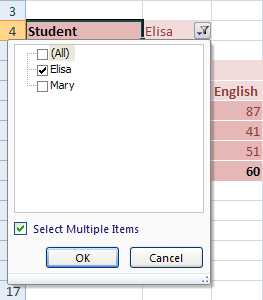
Now we have another student to select (we'll only use two students, for this tutorial). We could untick Lisa, and tick Mary instead. Then her scores would display.

The Subject and Month cells also have drop down lists. So we could view only January's scores, and just for Art and English, for example.
So this is a Pivot Table - a report that we can manipulate by selecting items from drop down lists. Let's make a start.
The first thing you need for a Pivot Table is some data to go in it. Instead of typing all the data out, you can simply grab ours. Go to this web page on our website and save the spreadsheet to your own hard drive:

Download the Data for the Pivot Table (Right click and select Save Link/Target As)

Once the spreadsheet is on your own computer, open it up. You should see this (If you get a warning across the top, click on Enable Editting):

The Pivot Table Data in an Excel Spreadsheet (New window)

Highlight the data that will be going in to your Pivot Table (cells A1 to D37).On the Excel Ribon, click the Insert tab. From the Insert tab, locate the Tables Panel.

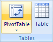
Pivot Tables are on the Tables panel in Excel 2007

On the Tables panel click Pivot Tables. The Create Pivot Tables dialogue box appears:

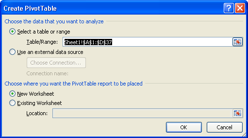
In the dialogue box above, the data that we highlighted is in the Table/Range textbox. You can select different cells by clicking the icon to the right of the Table/Range textbox. You can also specify an external data source, such as a text file, for the data in your Pivot Table.

We've selected a New Worksheet as the place where the Pivot Table will be placed. Click OK.
When you click OK, Excel presents you with a rather complex layout. The area on the right should look something like this one below:

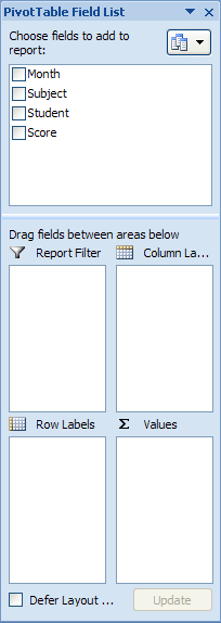
It helps to have a look again at what we're trying to create. Here's the completed Pivot Table again:

Now take a look at the Pivot Table Field List image again, the one above the completed pivot table. It has tick boxes for Month, Subject, Student, and Score. These are column headings from the original spreadsheet data. We've put the Month in cell A7 on our Pivot Table, Subject is in cell B6, Student is in cell B4, and Score is the Average scores in cells C8 to G10. You'll see how it works, though.

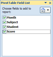
The idea is that you tick a box in the Pivot Table Field List, and then drag it to the four areas below. Excel will take care of the rest.

So, tick all four boxes in the field list:

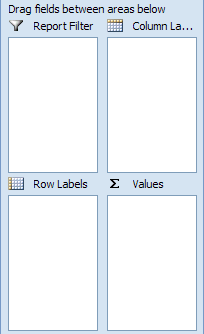
Excel will create a basic (and messy) Pivot Table for you. But we're going to put our 4 fields into the 4 areas below. Here are the 4 areas we can drag to:

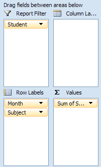
For the Report Filter, we want the name of a Student. For the Column Labels, we want the Subject, and for the Row Labels, we'll just have the Month. The Values will be the Average scores.

If you look at the Field areas after you have ticked all four boxes, however, you may see something like this: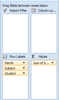

Month, Subject and Student have all been grouped under Row Labels. You can drag and drop these, though.

So click on Student in the Row Labels box. Hold down your left mouse button, and then drag it in to the Report Filter box. If you don't fancy dragging and dropping, simply click the Student item with your left button. From the menu that appears, select Move to Report Filter: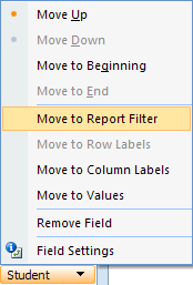

Your Field areas will then look like this:

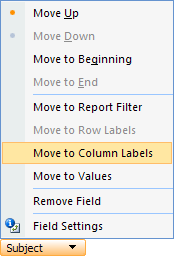
The Student item has been moved to Report Filter

Move Subject from Row Labels to the Column Labels area:

Your Field areas will then look like this:

The Pivot Table on your spreadsheet will look a lot different, too. It should be looking like this:

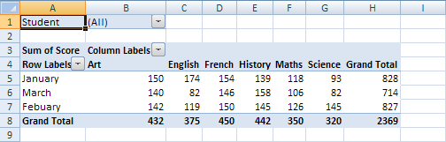
The reason why the scores from our Pivot Table are so strange is because Excel is using the wrong formula. It's using a Sum total when we want it to use an Average.

Here's the Pivot Table so far:

The numbers have all been added up. But we want averages, instead. To change the formula, click on Sum of Score under the Values field area:

You'll see the following menu:

Select, Field Settings (or Value Field Settings in Excel 2010). You'll then see the following dialogue box:

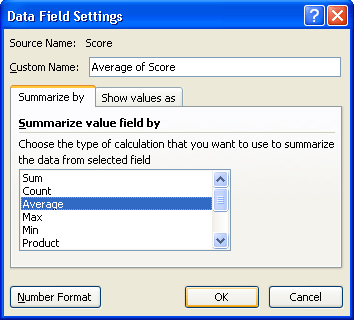
Change the Formula from Sum to Average, and then click OK. Your Average formula won't be formatted to any decimal places. So highlight you data. On the Home tab in Excel, locate the Number panel. Format your Averages so that it has no decimal places. Your Pivot Table will then look like this:

Almost there!

Look at cells A3, B3 and A4 above. These all have the not very descriptive names of Average of Score, Column Labels, and Row Labels. You can click inside of these cells and type your own headings, in exactly the same way as you would to enter text in a normal cell.

In the new version of the Pivot Table below, we have renamed these cells. We've also centred the data.

Only one thing left to do - spruce up the table by adding a bit of colour.

Click anywhere on your Pivot Table to highlight it. Now look at the Ribbon at the top of Excel . You'll notice a Design menu. Click on this to see the various design options.
The Pivot Table Style Options panel is interesting.

Select Banded Rows and see what happens. Now click Banded Columns.

Next to this panel, there are lots of Pivot Table Styles to choose from. Select one that catches your eye. Here's our finished Pivot Table again, only with a different Style: